use_of_gghmm2 • gghmm2

##Hidden Markov Model Hidden Markov model (HMM) is a statistical Markov model S where S is being model by a Markov process with hidden states. In other words S - which will be called the hidden state - can not be observed directly so we instead model on X which from now on will be called the observable states. Thus we learn about S at t=t₀ from X at t=t₀.

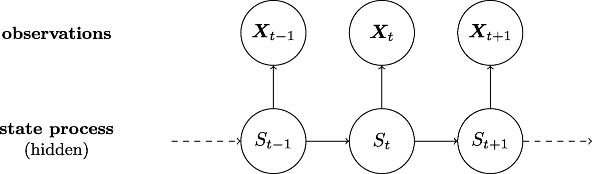
Overview of a Hidden Markov model

Overview of hmm on google

##The package

To see how the package works, we will cover a example of it, using the earthquakes data contained in the package. First we load that data set and build the model we will be using. We will be trying to fit a \(2\) state hidden markom model where the states emit from a poisson distribution. So we set emis_names to “dpois” to tell the model that we Here we use the HMM function to create the model.

X <- earthquakes$n
delta = c(0.5,0.5)
trans=matrix(c(0.9,0.1,0.1,0.9),2,2)
HM = HMM(initial_dist = delta,transmission = trans,
         emis_names = "dpois",parm1 = c(10,30) )
HM
#> [1] "This is a Hidden Markov model with 2 hidden states."
#> [1] "It has the initial distirbution of:"
#> [1] 0.5 0.5
#> [1] "It has the transmision matrix:"
#>      [,1] [,2]
#> [1,]  0.9  0.1
#> [2,]  0.1  0.9
#> [1] "State 1  has the emission function dpois with parameters 10"
#> [1] "State 2  has the emission function dpois with parameters 30"

Note that the print of the model, tells us how many hidden states the model has and the parameters values. As a alternative to using parm1 the user could also have used parameterlist = list(list(lambda=10),list(lambda=30)). However as we are only using one parameter for each distribution, then it is easier to just use parm1.

To use the forward and backward algorithms, the user can use the forward and backward functions. They just need to be supplied with the the model as HM and the data as X.

n = length(X)
FM = forward(HM=HM,X=X)
sum(FM[,n])
#> [1] 3.286743e-180
BM = backward(HM,X)

To find the probability of being at a certain state state at a time state_time, we can use state_prob. Again the user also need to provide a model as HMM and the data as X. Note that we cannot calculate the probability for a time bigger then the size of the data. So if we have a sequence of 10 observation, then state_time cannot be larger then 10.

state_prob(state = 1, state_time = 10, HM = HM, X = X)
#> [1] 7.169712e-09

The package also have both a local and global decoder. The local decoder function is called local_decoder and will return a vector of hidden states.

local_decoder(X,HM)
#>   [1] 1 1 1 1 1 2 2 2 2 2 2 2 2 2 2 2 2 2 2 1 1 1 1 2 2 2 2 2 2 2 1 2 1 1 2 2 2
#>  [38] 2 2 2 2 2 2 2 2 2 2 2 2 2 2 2 2 2 2 2 1 2 1 1 2 1 1 1 1 2 2 2 2 2 2 2 2 2
#>  [75] 2 2 2 1 1 1 1 1 1 1 1 1 1 1 1 1 1 1 1 1 1 1 1 1 1 1 1 1 1 1 1 1 1

The global decoder is called Viterbi and will return a list. The list contains the path with the highest probability of emitting X and the probability of getting this path.

viterbi(HM,X)
#> $path
#>   [1] 1 1 1 1 1 2 2 2 2 2 2 2 2 2 2 2 2 2 2 1 1 1 1 2 2 2 2 2 2 1 1 2 1 1 2 2 2
#>  [38] 2 2 2 2 2 2 2 2 2 2 2 2 2 2 2 2 2 1 1 1 2 1 1 2 1 1 1 1 2 1 1 2 2 2 2 1 1
#>  [75] 2 2 2 1 1 1 1 1 1 1 1 1 1 1 1 1 1 1 1 1 1 1 1 1 1 1 1 1 1 1 1 1 1
#> 
#> $path_prob
#> [1] 0.1137364

The forecast function allow the used to check what the probability of getting a state at a time in future will be. Here the user need to provide the state as a index as the variable pred_obs , and the time as pred_time.

forecast(2,10,HM=HM,X=X)
#> [1] 0.001134998

To last the user can use the Expectation–maximization algorithm to fit their data to a HMM. Here the user need to provide the data and a HMM object, which contain the initial guess for the parameters. The function will return HMM object, but now with the new parameters.

HM2 = em(HM,X)
#> [1] "Number of iterations: 35"
HM2
#> [1] "This is a Hidden Markov model with 2 hidden states."
#> [1] "It has the initial distirbution of:"
#> [1] 1.000000e+00 3.270886e-93
#> [1] "It has the transmision matrix:"
#>            [,1]      [,2]
#> [1,] 0.92837388 0.1190377
#> [2,] 0.07162612 0.8809623
#> [1] "State 1  has the emission function dpois with parameters lambda = 15.4203141191078"
#> [1] "State 2  has the emission function dpois with parameters lambda = 26.0170570907938"

A alternative example could be a fit of the normal distribution

HMN = HMM(initial_dist = delta,transmission = trans,
         emis_names = "dnorm",parameterlist = list(list(mean=10,sd=1),list(mean=20,sd=1)) )
HMN
#> [1] "This is a Hidden Markov model with 2 hidden states."
#> [1] "It has the initial distirbution of:"
#> [1] 0.5 0.5
#> [1] "It has the transmision matrix:"
#>      [,1] [,2]
#> [1,]  0.9  0.1
#> [2,]  0.1  0.9
#> [1] "State 1  has the emission function dnorm with parameters mean = 10, sd = 1"
#> [1] "State 2  has the emission function dnorm with parameters mean = 20, sd = 1"
HMN2 = em(HMN,X)
#> [1] "Number of iterations: 36"
HMN2
#> [1] "This is a Hidden Markov model with 2 hidden states."
#> [1] "It has the initial distirbution of:"
#> [1]  1.000000e+00 4.817079e-302
#> [1] "It has the transmision matrix:"
#>           [,1]      [,2]
#> [1,] 0.7678636 0.2912655
#> [2,] 0.2321364 0.7087345
#> [1] "State 1  has the emission function dnorm with parameters mean = 14.3443651201237, sd = 1.65298347289879"
#> [1] "State 2  has the emission function dnorm with parameters mean = 25.770101367033, sd = 2.05841704237087"